Jan. WTI 36.84 +0.53.
From RBN Energy, Dec. 10:
The CME/NYMEX Henry Hub contract for January delivery hit a 17-year low yesterday (December 10, 2015) of $2.015/MMBtu, 46 % below year-ago price levels. But US gas production has been humming along near 73 Bcf/d, more than 3.0 Bcf above a year ago and about 1.0 Bcf below the all-time high earlier this year. It’s a similar story for crude oil, with oil prices closing at $36.76/Bbl yesterday, but production hanging in there above 9 MMb/d. This is a testament to lower drilling service costs and producers’ ability to improve drilling productivity. But can productivity gains and drilling costs keep up with continually lower commodity prices? Today we look at how productivity gains and falling drilling costs are impacting producers’ rates of return.
Recap
In Part 1, we told the productivity story: how productivity improvements made production a formidable force in the market in 2015 in spite of substantial headwinds from low oil and gas prices, drilling budget cuts and falling rig counts. We showed how rig counts came off dramatically in correlation with prices this past year. But gas production volumes didn’t follow the rig count down. That’s because producers very quickly learned to do a lot more with a lot less.
To quantify drilling productivity in the context of gas, we showed various industry metrics, including drilling time, wells drilled per year per rig, 30-day average IP rate and IP additions per rig per year. We looked at these metrics over time for EOG Resources in the Eagle Ford play, which showed that EOG is now drilling wells in one-third the time it took in 2011, drilling three times more wells per rig each year, and producing double the volume from each well in its first 30 days. And all of that translates to five times more volume produced for every rig than in 2011. So there are fewer rigs operating but those rigs are much more prolific than they were in 2011 or even a year ago.
Using data from the Energy Information Administration’s Drilling Productivity Report, we then looked at average production per rig for entire basins, and found that EOG’s productivity gains are no exception. Productivity improvements are occurring in varying degrees across all the major shale basins, and for both oil and gas rigs.
Modeling Internal Rates of Return (IRRs)
Of course, the question then is what has all this done to producers’ internal rates of return (IRR) on their drilling investment and is it enough to sustain continuing growth? Cash flow returns are of high importance to producers, especially when oil and gas prices are down. But as we explained in It Don’t Come Easy Part 1, producers don’t make drilling decisions based simply on one commodity price threshold. Rather they look closely at break-even drilling economics and the resulting IRR to determine where to stop drilling and where to concentrate new activity. As you’d expect, the IRR, which takes into account both the relative prices of the hydrocarbons produced (oil, gas, NGLs) and well productivity, is not a static number for any given basin. To understand how IRRs have shifted with productivity gains in the past year, we ran drilling costs and other factors across major U.S. shale basins through our IRR model. As a reminder, in this exercise we are using half-cycle economics, which don’t include “sunk costs” such as lease costs, and in these cases both cost and price are held flat (no price or cost escalation factors). The model inputs, such as costs and production profiles (ie. type curves) are taken from representative wells in each basin. Against those inputs, we plug in the commodity prices. (see It Don’t Come Easy Part 2 for a detailed explanation of the model inputs, outputs and assumptions behind our analysis).
The following IRR snapshots provide a summary of our results for typical IRRs seen in oil, wet gas (NGLs) and dry gas plays for Fall 2014 versus today (December 2015), including several cost reduction scenarios at current price levels.
The Bottom Line – Producer Rates of Return
We start with IRRs back in Fall 2014 – the good ol’ days, when U.S. benchmark West Texas Intermediate (WTI) crude oil price was $90/Bbl and Henry Hub natural gas was at $3.75/MMBtu. We first showed these results It Don’t Come Easy Part 3. Here they are again in Figure 1 below.
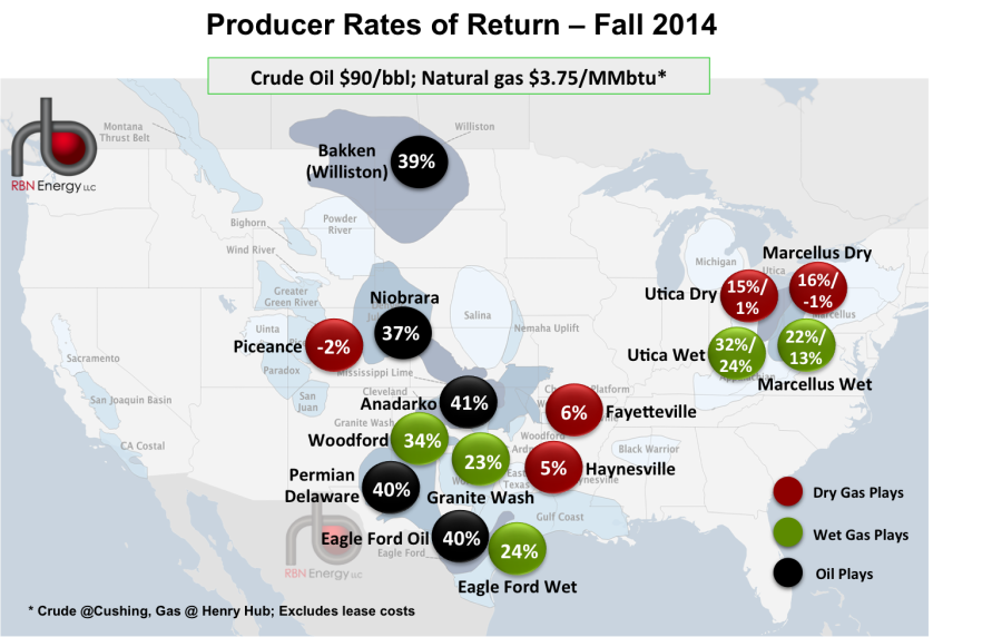
Figure 1; Source: RBN Energy (Click to Enlarge)
If you’ll recall, at those prices, crude oil plays (black circles) offered returns near 40%. Liquids-rich gas plays (green circles) offered returns in the mid-20%. And dry gas plays (red circles) offered mostly single-digit but still positive IRRs, with the exception of the Marcellus and Utica, where some producers could be seeing higher IRRs around 15%. Note that there are two IRR numbers in the Marcellus and Utica circles. In the first scenario (top number in the circles), we assume producers have the proximity or available transport capacity to get to the higher priced Columbia Gulf TCO point. In the second scenario (bottom number in the circles), we assume producers are stuck with weaker basis differentials (lower prices) typical of several capacity-constrained locations in that region, including the Dominion South pricing point....MORE