From Six-Figure Investing, Mar. 10, 2017:
It’s not obvious (at least to me) that volatility theoretically scales with the square root of time (sqrt[t]). For example if the market’s daily volatility is 0.5%, then the volatility for two days should be the square root of 2 times the daily volatility (0.5% * 1.414 = 0.707%), or for a 5 day stretch 0.5% * sqrt(5) = 1.118%.
This relationship holds for ATM option prices too. With the Black and Scholes model if an option due to expire in 30 days has a price of $1, then the 60 day option with the same strike price and implied volatility should be priced at sqrt (60/30) = $1 * 1.4142 = $1.4142 (assuming zero interest rates and no dividends).
Underlying the sqrt[t] relationship of time and volatility is the assumption that stock market returns follow a Gaussian distribution (lognormal to be precise). This assumption is flawed (Taleb, Derman, and Mandelbrot lecture us on this), but general practice is to assume that the sqrt[t] relationship is close enough.
I decided to test this relationship using actual S&P 500 data. Using an Excel based Monte-Carlo simulation1 I modeled 700 independent stock markets, each starting with their index at 100 and trading continuously for 252 days (the typical number of USA trading days in a year). For each day and for each market I randomly picked an S&P 500 return for a day somewhere between Jan 2, 1950 and May 30, 2014 and multiplied that return plus one times the previous day’s market result. I then made a small correction by subtracting the average daily return for the entire 1950 to 2014 period (0.0286%) to compensate for the upward climb of the market over that time span. Plotting 100 of those markets on a chart looks like this:
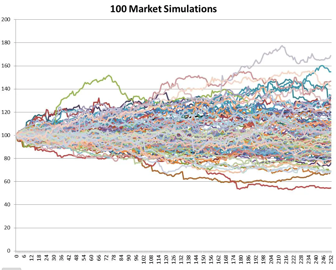
Notice the outliers above 160 and below 60.
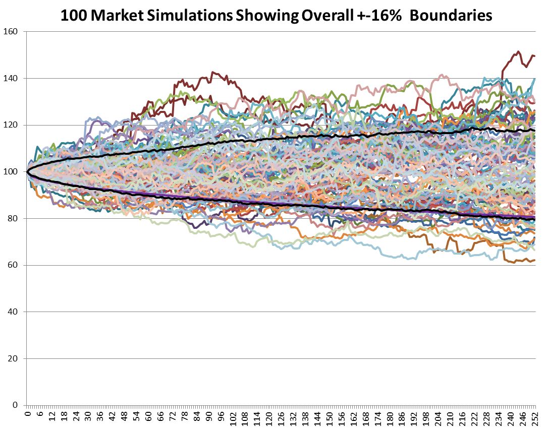
Volatility is usually defined as being one standard deviation of the data set, which translates into a plus/minus percentage range that includes 68% of the cases. I used two handy Excel functions: large(array,count) and small(array,count) to return the boundary result between the upper 16% and the rest of the results and the lowest 16% for the full 700 markets being simulated. The 16% comes from splitting the remaining 32% outside the boundaries into a symmetrical upper and lower half.
Those results are plotted as the black lines below.
...MORE